

TL;DR version. Loaded AWS detailed billing reports to BigQuery. Generic Queries are available here in this repo: bit.ly/2iu3R6G. Send pull requests. Redash was used to visualize.
AWS default billing and cost management dashboard is already pretty informative. The cost explorer allows analyzing the data by custom date ranges, grouping by select services etc. But there are much more deeper insights hiding in your detailed billing reports, if you know where to look. Example, you find that there is a sudden spike in data transfer out costs. Did someone took control of your Jenkins server and using it for bitcoin mining? Or was it a legitimate usage? How do you identify which resource is causing the spike? With detailed billing reports loaded to a database, finding answers to questions like these and much more is just few simple SQL queries away.
At any given point, we manage not less than 50 AWS accounts of varying sizes for our clients. Looking at the frequent questions related to billing that we deal with, we set out building custom dashboards that refresh everyday with latest billing data using ReDash. This post explains loading a sample report to BigQuery and some sample queries are included.
AWS billing and usage reports can directly be uploaded to RedShift and then QuickSight can visualize them. Why not use Athena + QuickSight or RedShift + QuickSight? Well, I have used both Athena and RedShift extensively for other use cases and they are awesome at what they do. But for this use case, they seemed not a good fit. I will explain why.
AWS billing report is a CSV file that gets updated depending on the interval you choose. When I created an external table pointing to one of the billing reports using LazySimpleSerde, I ended up with data that looks like this:
rateid subscriptionid pricingplanid
"12334317" "232231735" "915879"
"12334331" "232231735" "915879"
Now that is problematic. Looks like athena doesn’t strip the quotes out of data when it renders it. This makes it difficult to aggregate the costs. There are workarounds. You could use sed to replace doublequotes from CSV before creating external table OR you could write your query like this to strip quotes on the fly and then aggregate SELECT SUM(CAST(REPLACE(blendedcost, '"', '') AS FLOAT)) as TotalCost - but after running into a couple of issues related to conversion, I gave up on Athena. Next RedShift - since its a full fledged columnar database, none of these would be a problem, but owning RedShift cluster comes with certain management overhead. I didn't want take the trouble of deleting the cluster everyday and recreate to save costs. So I chose BigQuery, which is zero management, crazy fast, we just pay for the storage and first 1 TB of data processed during query execution is free.
So with that out of the way, let’s get to the step by step.
What do you need to get started?
If you have come this far, I assume you already know what detailed billing reports are and how to enable them etc. If you don’t, visit this documentation page. You need the following.
Access to the S3 bucket where detailed billing reports are stored
A Google cloud project and a google storage bucket.
BigQuery enabled.
A small ec2 instance to install and host
redash
Download Report from S3 and upload to Google Bucket
- Create an IAM policy granting read-only access to the target S3 bucket for a user.
{ "Version": "2012-10-17", "Statement": [ { "Effect": "Allow", "Action": "s3:*", "Resource": "arn:aws:s3:::myBillingBucket/*" } ] }
- Setup
AWS Clion a VM from which your scripts will run.
pip install awscli
Configure
aws cliusing secret and access keys of a user you attached the above readonly policy to. Instructions for configuringaws cliare here.Find the last updated file and download. The bucket will likely have multiple files. Since we know only last few characters of the report name change based on the month, we can grep by file name pattern, sort and look at the last modified file.
aws s3 ls s3://mybillingbucket/ | grep xxxxxxxx6559-aws-billing-detailed-line-items-with-resources-and-tags-* | sort | tail -n 1 | awk '{print $4}'
- Copy the file locally and unzip.
FileName="$(aws s3 ls s3://mybillingbucket/ | grep xxxxxxxx6559-aws-billing-detailed-line-items-with-resources-and-tags-* | sort | tail -n 1 | awk '{print $4}')"
aws s3 cp s3://mybillingbucket/$FileName /bills/client1/$FileName unzip /bills/client1/$FileName -d /bills/client1/
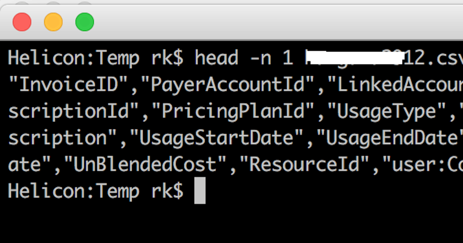
- Now that you have the latest bill, you might want to take a look at the columns you have so that you can come up with the schema for creating the table in BigQuery. these files tend to be relatively big, so use head to take a look at the columns.
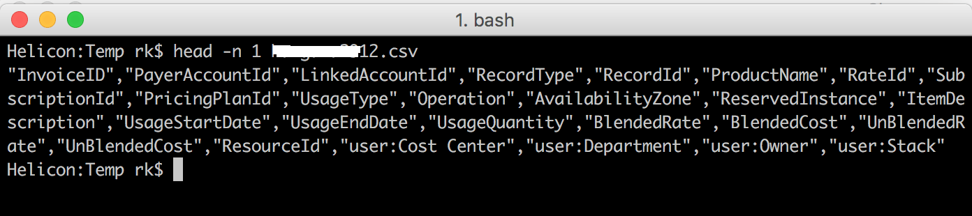
Make a note of these in a text file. This can be used to created the schema definition while creating the table for the first time.
BigQuery can load gzipped CSV files from a cloud storage buckets. To speed up uploads and to make sure you dont pay much in data out costs from your AWS VM, gzip the file. Our
FileNamewill generally look likesomething.csv.zip. After unzipping it, we need to make changes to our FileName and remove those last 4 characters.zip
FileNameCSV=${FileName::-4} gzip < /bills/client1/$FileNameCSV > /bills/client1/$FileNameCSV.gz
Next, setup Google Cloud command line utilities for interacting with storage and bigquery. Check documentation for detailed steps.
I am assuming you already have a google cloud bucket created and command line utilities configured. Upload the gzipped file to target google cloud bucket.
gsutil cp /bills/client1/$FileNameCSV.gz gs://powertracker/client1/$FileNameCSV.gz
Create BigQuery Dataset and Load Data
Installing Google Cloud SDK will also take care of BigQuery’s command line utility,
bq.Create a BigQuery dataset (kind of like the database) from either UI or using command line utility. Here is a quickstart that will help you with this.
Now if you recollect in the previous section, we saved the schema definition in a text file. That will come in handy now. Create a json schema file with the columns from your csv and use it as a schema definition file to create the table. An example schema definition file will look like this:
[ {"name": "InvoiceID", "type": "string", "mode": "nullable"}, {"name": "PayerAccountId", "type": "string", "mode": "nullable"}, {"name": "LinkedAccountId", "type": "string", "mode": "nullable"}, {"name": "RecordType", "type": "string", "mode": "nullable"}, {"name": "RecordId", "type": "string", "mode": "nullable"}, {"name": "ProductName", "type": "string", "mode": "nullable"}, {"name": "RateId", "type": "string", "mode": "nullable"}, {"name": "SubscriptionId", "type": "string", "mode": "nullable"}, {"name": "PricingPlanId", "type": "string", "mode": "nullable"}, {"name": "UsageType", "type": "string", "mode": "nullable"}, {"name": "Operation", "type": "string", "mode": "nullable"}, {"name": "AvailabilityZone", "type": "string", "mode": "nullable"}, {"name": "ReservedInstance", "type": "string", "mode": "nullable"}, {"name": "ItemDescription", "type": "string", "mode": "nullable"}, {"name": "UsageStartDate", "type": "string", "mode": "nullable"}, {"name": "UsageEndDate", "type": "string", "mode": "nullable"}, {"name": "UsageQuantity", "type": "string", "mode": "nullable"}, {"name": "BlendedRate", "type": "string", "mode": "nullable"}, {"name": "BlendedCost", "type": "string", "mode": "nullable"}, {"name": "UnBlendedRate", "type": "string", "mode": "nullable"}, {"name": "UnBlendedCost", "type": "string", "mode": "nullable"}, {"name": "ResourceId", "type": "string", "mode": "nullable"}, {"name": "user_CostCenter", "type": "string", "mode": "nullable"}, {"name": "user_Department", "type": "string", "mode": "nullable"}, {"name": "user_Owner", "type": "string", "mode": "nullable"}, {"name": "user_Stack", "type": "string", "mode": "nullable"} ]
The number of columns in your file may differ based on the cost allocation tags you have enabled. If you notice the above schema, all columns that start with
user_are tags from this particular account. I also chose all data types as string because I wanted to avoid load failures and anyway BigQuery is pretty complete with conversions.Next, go ahead and load the data to your table. In the command below,
powertrackeris my dataset (database) and the name of target table ispowertracker.client1.clien1schema.jsonos the file we generated above
bq load --schema=/bills/client1schema.json powertracker.client1 gs://powertracker/client1/$FileNameCSV.gz
Note that when you turn all of these steps into a script, the bq load might fail the second time because the table with name
client1already exists from yesterdays load. So all you need to do is,bq rm powertracker.client1and then run the load command.Just like Amazon Athena, BigQuery too can run queries on files stored on Google Cloud Storage via external tables. I tried this but I decided to go ahead with loading data than using federated tables. I think the whole file gets processed for each query when created as federated table (I was using gzipped target, it may behave differently with plain CSV, I am yet to test it). The external tables don’t take advantage of columnar nature of BigQuery and they are a little bit slower compared to when you load data.
Queries, Insights and ReDash
Now that we have a process to load data from S3 to BigQuery via Google Cloud Storage bucket every day, its now time for the exciting part. Running queries and gaining insights. I created a public repo on github with some of the generic queries that I came up with. Feel free to fork and send pull requests. Here is the repo.
Lets say I would like to find why there is a sudden surge in data out costs. I first need to identify what usage types are available so that I can filter by it. If you do a SELECT DISTINCT usagetype, you will note that most of the usagetypes related to data out have something in common - the word `'Out-Bytes', so here is the query.
#If using legacy SQL, change FLOAT64 to FLOAT.
SELECT SUM(CAST(blendedcost AS FLOAT64)) AS Cost, resourceid
FROM powertracker.client1
WHERE usagetype LIKE '%Out-Bytes%'
GROUP BY resourceid
ORDER BY Cost DESC
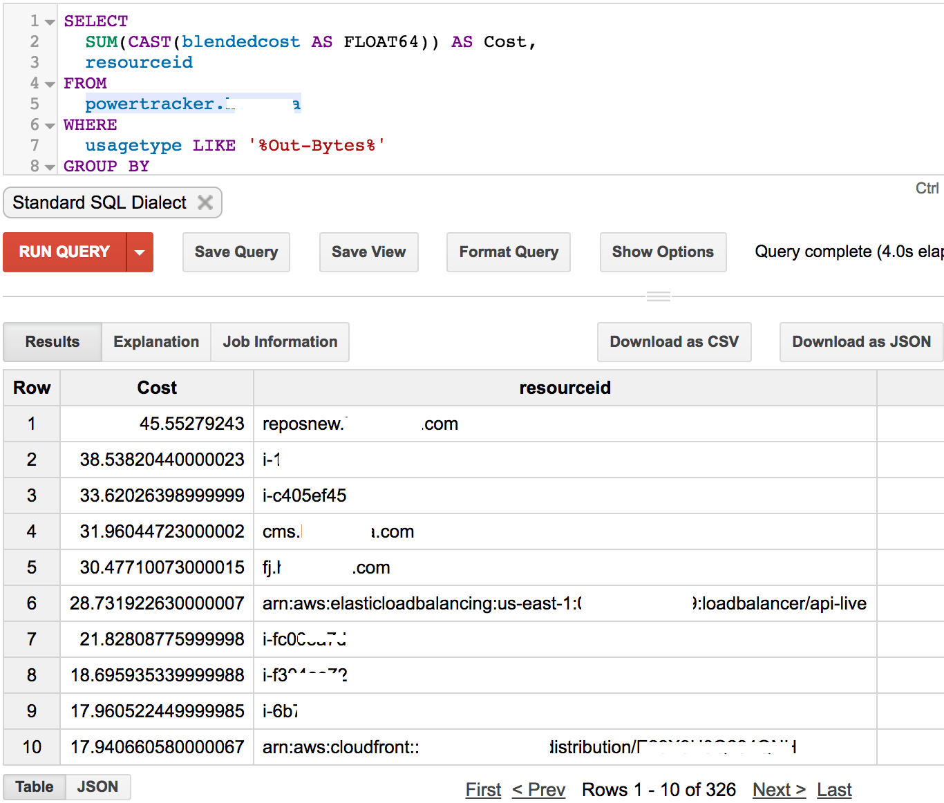
And boom — it took 4 sec. Now I exactly know which servers/CloudFront distributions/ELBs are responsible for the data out costs including their resourceids.
Next, if I would like to know which internal services/tags are contributing to most of the bill, here is the query. We need to make sure that InvoiceTotal, StatementTotal etc are excluded from aggregation, otherwise you will end up with misleading numbers.
SELECT SUM(CAST(blendedcost AS FLOAT)) AS Cost,
user_costcenter,
user_department,
user_owner,
user_stack
FROM powertracker.client1
WHERE RecordType NOT IN ('InvoiceTotal', 'StatementTotal', 'Rounding')
GROUP BY 2, 3, 4, 5
ORDER BY Cost DESC;

What if I would like to find the cost by internal services/tags for a specific day? Well thats easy. here we go:
SELECT SUM(CAST(blendedcost AS FLOAT)) AS Cost,
user_department
FROM powertracker.client
WHERE DATE(TIMESTAMP(usagestartdate)) = '2017-01-01'
GROUP BY user_department,
ORDER BY Cost DESC;

This is barely scratching the surface. There is much more you can do once the data is available on BigQuery. Go ahead and take a look at all the queries in the github repo and play around. If you figure out more queries that would help gaining more insights, please send a pull request :)
So where does ReDash fit in? Once you setup a daily load and write some queries — wouldn’t it be awesome if you can visualize it? ReDash can talk to BigQuery and it allows creating multiple dashboards with access control enabled to a groups of people.
Setting up redash is a breeze. Just provision an Ubuntu machine and get this installation script. Run it. Done!
Connect to ReDash and configure your data source

Go to Google Cloud Console, IAM&Admin page and then create a service account that will be used by redash to connect to BigQuery
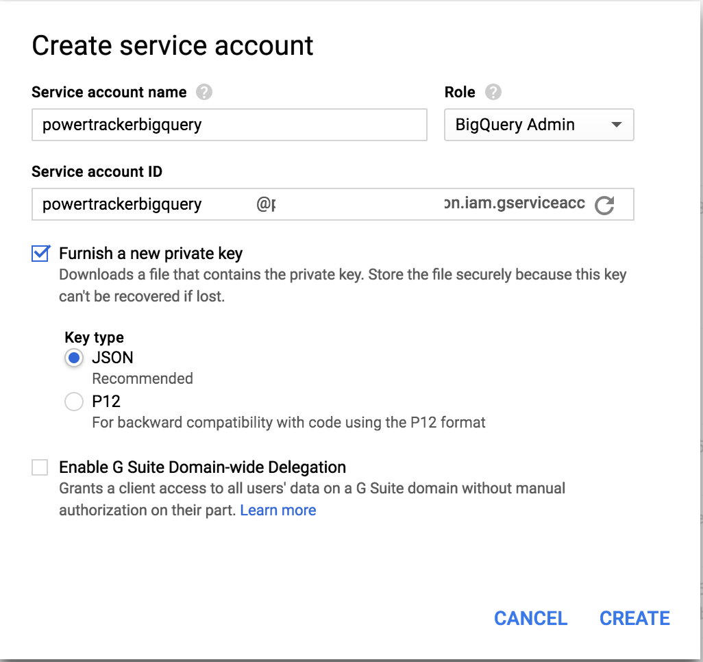
That should download a JSON key. Come back to ReDash datasource config page and upload the key. That’s it. You can now open a new Query window on ReDash and test a Query.

In the next series of posts, I will write about creating useful dashboards using redash, loading AWS usage reports along with billing reports and bringing all of this together as a unified dashboard.
Meanwhile, I hope you found this useful. Happy cost analytics! :)
Originally published at blog.powerupcloud.com on January 8, 2017.